William Fried, Andrew Fu, Matthieu Meeus, Emily Xie
Overview
Introduction
Latent Dirichlet Allocation (LDA) is a popular unsupervised, Bayesian hierarchical model commonly applied to topic modelling. Given a list of documents, a prespecified number of topics, and several hyperparameters, LDA assigns each word in the corpus to a particular topic. Based on these assignments, LDA learns two main features of the corpus:
It identifies each topic by ranking the importance of each word in the vocabulary to the given topic;
It weighs the contribution of each topic to the content of each document.
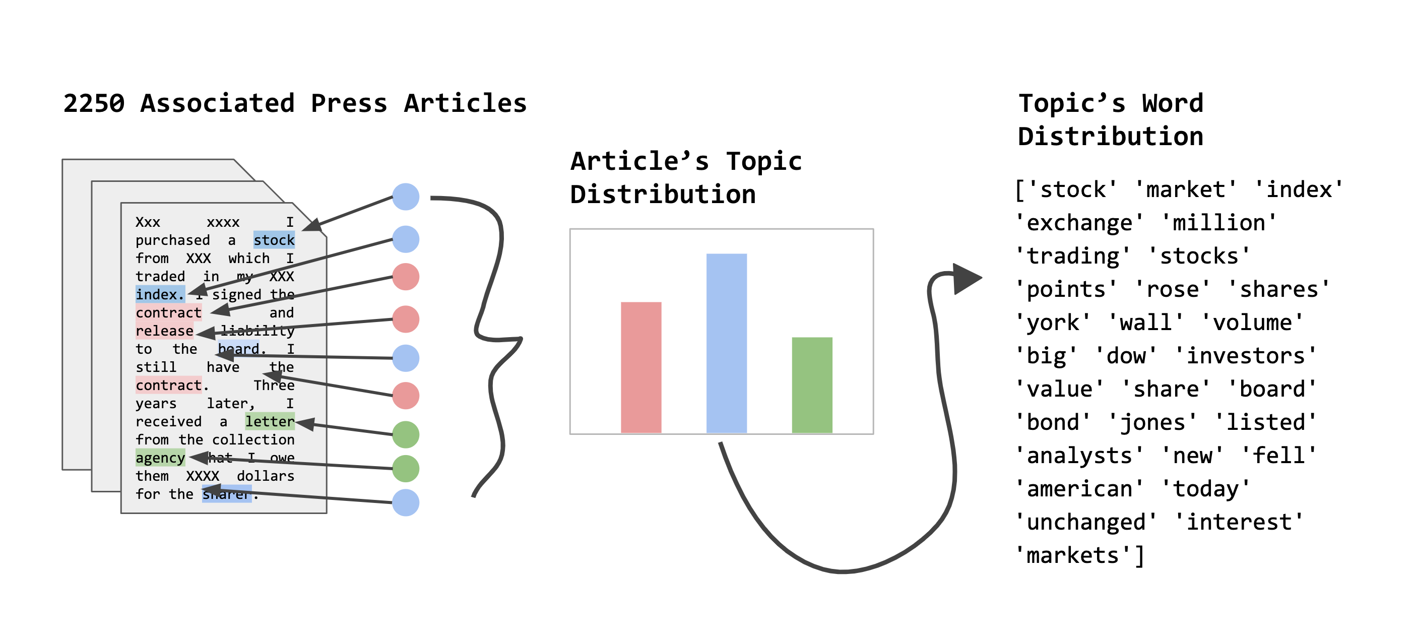
The figure below illustrates how LDA results in a topic distribution for each document. To the right, we show a list of 20 words that we have found associated with a selected topic in the distribution. Clearly, the results make sense, as all words displayed are thematically related––in this case, the stock market. Because LDA is so widely used and well documented, we omit the details of the generative model and direct curious readers to the original paper here [1]. This project will focus on the parallelization of LDA; our source code is available on Github (link)
Inference for LDA
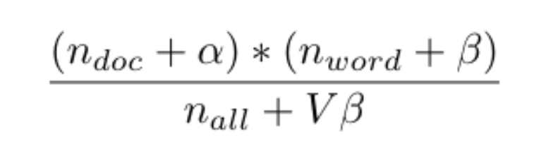
There are several procedures used to infer the distribution of words per topic and the distribution of topics per document. The two most common approaches are 1) variational Bayesian inference and 2) collapsed Gibbs sampling. For this project, we focused on parallelizing the collapsed Gibbs sampling algorithm (CGS). CGS works as follows: first, every word in each of the documents is randomly assigned to one of the T topics. After this initialization step, the first iteration of CGS is performed where each word in the corpus is reassigned to a new topic. For an arbitrary word w in document d, this is achieved by sampling from a categorical distribution, where the unnormalized weight associated with each topic t is:
where n_doc represents the number of words in document d assigned to topic t, n_word represents the number of times word w is assigned to topic t across all documents, n_all represents the number of words in the corpus that are assigned to topic t, α and beta are the LDA hyperparameters, and V is the vocabulary size.
As CGS is a Markov Chain Monte Carlo (MCMC) algorithm, the distribution of assignments, in theory, converges to the posterior distribution of topic assignments. In practice, iterations are performed until the algorithm converges (based on likelihood or any number of metrics) and the assignments are used to construct the topics.
There are several quantitative metrics that can be used to assess the quality of a topic model. The first is a perplexity score, which approximates the likelihood of the words in a held-out set of documents. However, while likelihood-based metrics are statistically principled, it has been shown that LDA models that are optimized by minimizing the perplexity score often do not align with human judgement about what constitutes a logical topic. Topic coherence, a much more intuitive measurement, is presented here [2]. The basic idea is that if the model believes that two arbitrary words, i and j, are among the most common words in a given topic, then these two words should often appear together in the same document. One way to quantify this is to calculate the conditional probability of word j appearing in a document given that word i appears in the document. By the definition of conditional probability, this is equal to the total number of documents in which words i and j coappear divided by the total number of documents in which word i appears. To calculate the topic coherence of a single topic, the log of this conditional probability is computed for all pairs of words i and j among the M most probable words in the given topic, and these calculations are summed together. Finally, because there are multiple topics, this procedure is repeated for each topic and the average of these topic coherences is taken to be the overall topic coherence measurement. The CGS algorithm has likely converged when this topic coherence metric does not change significantly between consecutive iterations. Once the CGS has converged, the final step is to calculate the distribution of words per topic and the distribution of topics per document.
The posterior distribution of words for each topic t is a V-dimensional Dirichlet distribution with the following parameter for each word w in the vocabulary:
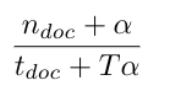
The posterior distribution of topics for each document d is T-dimensional Dirichlet distribution with the following parameter for each topic t:
where t_doc represents the total number of topics assigned in document d.
Based on the properties of the Dirichlet distribution, the probability of the cth category is proportional to the cth parameter. This means that the most common words associated with a topic and the most common topics associated with a document are those that have the highest corresponding Dirichlet parameters.
Serial Implementation
The serial version of CGS, where one process is assigned all of the documents, follows naturally from the general procedure described above. First, the three counts described above are initialized to zero. The next step involves iterating over each document in the corpus and over every word in each document and randomly assigning each word to one of the T topics specified. After word w is assigned to topic t in document d, the three corresponding counts are incremented by one; namely, the number of words in document d that are assigned to topic t, the number of times that word w is assigned to topic t across all documents, and the number of words assigned to topic t across all documents. Overall, the time complexity of this initialization step is O(d\*w) where d represents the number of documents in the corpus, and w represents the average number of words per document.
At this point, we're ready to begin performing CGS. Just as with the initialization step, this involves iterating over each word in each document. The process of reassigning word w in document d that was previously assigned to topic t_old consists of three parts. First, word w is unassigned from topic t_old, which is represented by decrementing the three relevant counts. Next, the unnormalized weight is determined for each of the T topics by calculating the expression defined above, and a random topic, t_new, is sampled from the resulting categorical distribution. Finally, word w is assigned to topic t_new, which is represented by incrementing the three relevant counts. After each iteration, the topic coherence metric described above is calculated and compared to the value of the previous iteration. Just as with the initialization step, because each iteration involves looping through each word in the corpus, the time complexity of each iteration is O(d\*w).
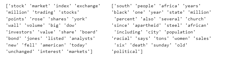
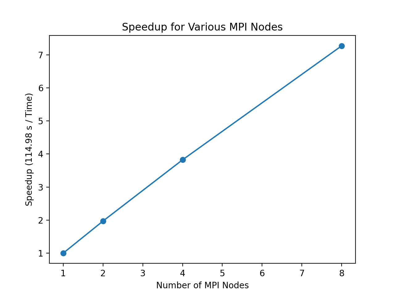
This serial implementation has been tested on a sample of approximately 2,000 news articles. The top words of two topics are listed below and a plot the overall topic coherence is plotted over number of iterations of the CGS.
Clearly, the algorithm is able to group a set of words that make intuitive sense in the context of one particular topic. In this case, the topic on the left seems to be centered around the theme of the stock market, while the one on the right relates to South-African politics. The plot further shows how the CGS algortihm converges towards a constant value for the average topic coherence.
A Parallel Paradigm
The Need for HPC and Big Data
While the serial version of CGS described above is straightforward to implement, it scales linearly with the number of documents in the corpus. This means that performing LDA on a moderately large number of documents is highly computationally expensive. To get a sense of this, we implemented a serial version of LDA in Python and applied it to a toy dataset of approximately 2,250 Associated Press articles (these articles can be found here). The algorithm converged after 10 iterations and took 380 seconds to run. Assuming it would take the same number of iterations to converge, this level of performance indicates that it would take many hours to run LDA on a more realistic corpus that contains hundreds of thousands––or even millions––of documents.
Therefore, we sought to parallelize this algorithm by applying the big compute tools of MPI and OpenMP. We wrote our implementation in Cython because Python's GIL prevents multithreading, which is needed to run OpenMP. An added benefit of Cython is that it compiles down to C (rather than being interpreted, as with vanilla Python), which gave us an automatic boost in performance.
We applied our parallelized version of CGS to Stanford's DeepDive patent corpus (accessible at this this link.), which contains approximately 2.5 million patent grants submitted to the United States Patent and Trademark Office since 1920. For our project, we used roughly 360,000 of these patent documents. Because each patent document needs to be preprocessed before being fed into the CGS algorithm, this also presents a big data problem. To parallelize this process, we turned to Spark.
Parallel Design
Parallelizing the CGS algorithm is not a trivial task. This is the case because the categorical distribution that is used to reassign each word depends on the three count values that are constantly changing as words are being processed. In other words, setting up the proper categorical distribution depends on knowing the topic assignment of other words in the corpus at the given time. However, all hope is not lost because setting up the categorical distribution depends on knowing only a subset of the topic assignments of the other word in the corpus. Therefore, our goal is to find a way to reassign multiple words at the same time such that the topic assignment of one of these words doesn't affect, or only slightly affects, the topic assignments of the other words. Each word assignment relies on the document-assignment (n_doc), word-assignment (n_word) and topic-assignment (n_all) counts; we discuss how to manage each of these counts in turn. Note that the approach we describe below is a modified version of Nomad LDA as discussed by Yu et al. as presented here [3].
Of the three counts, the document-assignment count is the easiest to handle. If we ensure that no two words from the same document are reassigned simultaneously, then the document-assignment counts corresponding to each word will be independent. We can easily achieve this by assigning a subset of the documents in the corpus to multiple nodes such that each document is “owned” by one of the nodes. This guarantees that when a node reassigns a word in a given document, it has access to the exact document-assignment count and does not conflict with any of the other nodes.
Dealing with the word-assignment count is more complicated. The issue is that if multiple nodes reassign multiple occurrences of a given word in the corpus, then the word-assignment count will be different across the nodes. Therefore, we must find a way to ensure that only one node can process a given word in the vocabulary at any point in time. This can be achieved by creating a tuple for each word that contains the word itself (e.g. 'invention') and its associated topic counts. Next, we enforce a system where only the node that possesses the tuple for word w has permission to reassign word w (just as a student in elementary school needs to possess a bathroom pass to walk in the hallways during class). Because there is only one tuple for each word in circulation, this guarantees that no two nodes can simultaneously reassign the same word. Of course, each node most likely has documents that contain a given word in the vocabulary, which means that each node must periodically be in possession of each of these tuples.
This can be achieved as follows: upon initialization, each node is assigned a some subset of the tuples such that the workload is spread out as evenly as possible. (While the workload associated with each tuple is proportional to the frequency of the associated word in the corpus, assuming there are far more words than nodes, the law of large numbers suggests that the high-frequency and low-frequency words will balance out such that the workload is roughly the same for each of the nodes.) These tuples are then placed in a queue, a first in, first out data structure. Each node then pops the first tuple off of its queue and processes it by reassigning each occurance of the given word across the documents allotted to it and updating the word-assignment count to reflect these reassignments. Once this has been completed, each node passes off this updated tuple to the next node (e.g. node 0 to 1, 1 to 2, 2 to 3, 3 to 0), which, in turn, proceeds to push this tuple onto its own queue. This next node now has the exact word-assignment count needed to properly reassign the occurrences of the word in its document. Each node is now free to pop the next tuple off of its queue and repeat the same procedure.
Finally, we need to handle the topic-assignment count. At first this may seem like a futile proposition because every word that is reassigned modifies the topic-assignment count, which means it would be impossible for each node to keep an accurate topic-assignment count. However, all hope is not lost as CGS is an MCMC algorithm. This means that we only need to converge to the same posterior distribution. This means that even if each node only has access to an approximate topic-assignment count, the sampling will still converge, perhaps taking more iterations, as long as the count is updated periodically. (The fact that the topic-assignment count for each topic is large (on average the total number of words in the corpus divided by the number of topics), coupled with the fact that this count generally does not change dramatically from between re-assignments means that the approximate categorical distribution set up by each node should differ only minimally from the optimal categorical distribution that is used in the serial implementation.)
The updating scheme works as follows: during initialization, each node randomly assigns the words in its alloted documents. Next, the topic-assignment counts of each node are summed together to produce an overall topic-assignment count that reflects the topic assignment of each word in the corpus. This global topic-assignment count is then disseminated to each of the nodes. The nodes do not modify this count, as it serves as a snapshot of what the global topic-assignment count is at the beginning of the iteration. Instead, each node creates a new data structure that maps each topic to the change in the number of words assigned to the given topic, and initializes these counts to zero. When the iteration begins and words are reassigned, the node increments and decrements these counts as appropriate, such that at the end of the iteration this mapping reflects the net change in the topic assignments of the words in the node's alloted documents (e.g. if 10 words were assigned to topic 1 at the beginning of the iteration and 5 of these words were reassigned to topic 2 while 3 words that were initially assigned to topic 2 were reassigned to topic 1, then the net change would be -5 + 3 = -2 for topic 1 and 5 - 3 = 2 for topic 2). Once the iteration is complete, this net change count is summed across all the nodes. The resulting count represents the net change in the topic assignments across the entire corpus, and is broadcasted to each of the nodes. Next, each node adds this count to the unchanged topic-assignment count, which now serves as an updated snapshot of the global topic-assignment count. Finally, the net change count is reset to zero in preparation for the next iteration.
Parallel Implementation & Performance
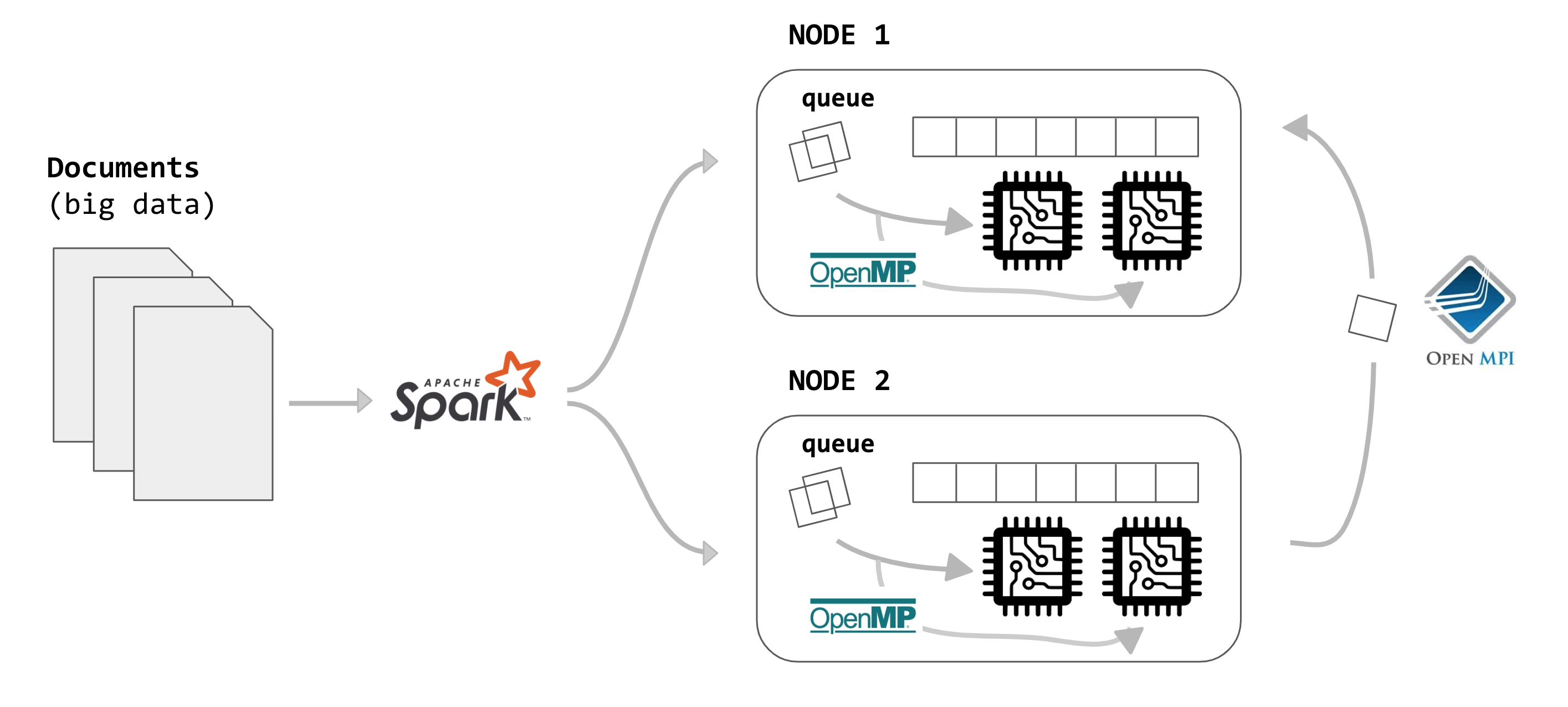
Overview
The following figure illustrates the overall parallelization scheme that will be implemented. First, we'll use Achache Spark to preprocess the large PATENT dataset, run on multiple nodes withing an EMR cluster. Once the data is correclty preprocessed, we distribute the results over multiple nodes in our cluster. These nodes will then sample with the Gibbs Sampling algorithm, and communicate the intermediate results to one another using MPI. Within each node, we can achieve further speedup by leveraging OpenMP.
The next paragraphs will further elaborate on the detailed implementation of the Spark preprocessing, MPI and OpenMP.
Document Pre-Processing
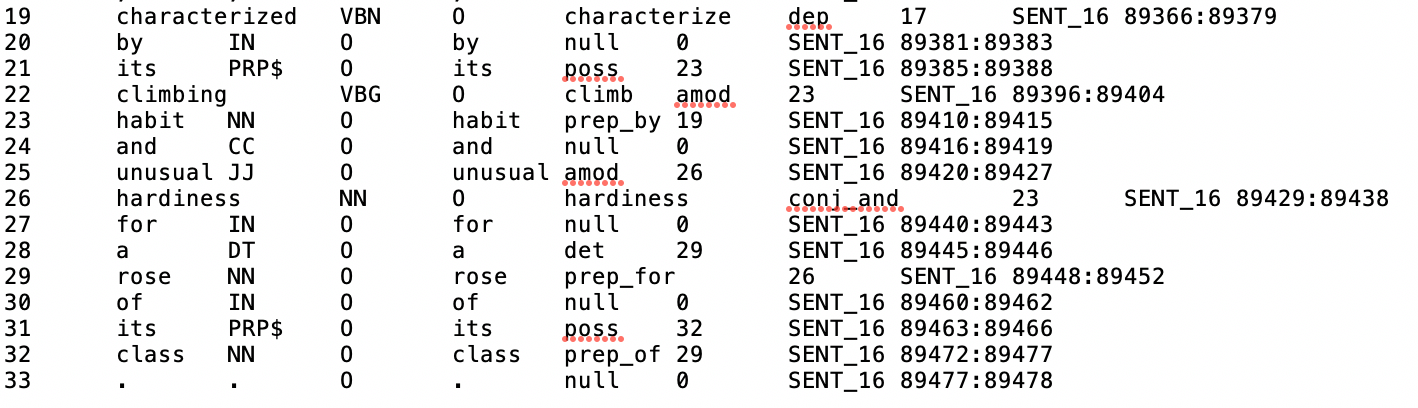
As outlined above, the first step of the implementation was to download the patents documents, preprocess them and convert them to a format that could easily be ingested by the parallelized CGS algorithm. Each patent document came in the following format:
As shown above, the actual words of the patent are listed in the second column, while the rest of the columns contain additional information that may be useful to other natural language processing tasks. (Most of these patent documents were written before the advent of modern computers, so the majority of them are transcribed using optical character recognition software. As a result, some of the words were transcribed incorrectly (e.g. “w” might be transcribed as “vv”)).
Thus, the first step was to extract these words from the patent documents. Our goal was to write the sequence of words in each patent document as a separate line in a text file, as this format would allow us to easily create an RDD using SparkContext’s textFile method. We used Python's multiprocessing module to speed up this process.
Because multiple workers cannot write to a file at the same time, we cannot simply use the mp.Pool().map function to process each patent document independently. Instead, we created the following setup: first, we set up a queue using the multiprocessing Manager, so that the workers can communicate with each other. Then, we task one of the workers in the pool with constantly monitoring this queue and writing each element as a new line in a text file (this was accomplished using the apply_async method). Next, we call the starmap method to pass each patent document, along with a reference to the queue, to each of the remaining workers in parallel. To process a given patent document, each of these workers iterates through the lines and extracts the word in the first column. It then converts the word to lowercase; removes any special characters such as dashes and punctuation marks; and ignores any words that are stopwords (as defined by the Natural Language Toolkit library), consist of fewer than four characters or contain any numeric characters. The requirement that each word be at least four characters long was added because many of the words that were misread by the optical character recognition (OCR) software contain three or fewer characters and are inscrutable. All of the surviving words are then concatenated into one long string and pushed onto the queue, so that they can be written to the text file. We then uploaded this text file to an AWS S3 bucket for further processing. The source code for this approach can be found here.
As outlined in the project design, the first step in the parallelization of LDA in this project is the preprocessing of the documents using Spark. Recall that our test input is the Google PATENT dataset (publicly available from Stanford DeepDive). The entire dataset (428 GB) contains over 2 million patent grants issued in the US since 1920. For the purpose of this project, only a subset of about 360,000 documents was used. Given that the computational complexity of the LDA algorithm is proportional to the number of documents, we decided that this was enough to justify the need for parallel processing and would clearly illustrate the impact of our parallelization efforts.
The patents are given as NLP files spread over multiple folders. The Spark pipeline needs to process this raw input to the exact input format required by the CGS algorithm. Specifically, it needs to:
Read in all the words over all the patents.
Count all the occurences of each word per document.
Aggregate all the filtered words and compose the vocabulary to be considered by the algorithm. In this step, a minimum of total number of occurences of a word over all documents and a minimum individual document occurences will be applied to all words. As such, a coherent topic distribution can be reached.
Write two main outputs:
The entire vocabulary, where each word is matched to its index.
A dictionary mapping each document to a list of all the words from the vocabulary that appear in that document and its corresponding count.
The serial implementation of this preprocessing for the considered dataset was estimated to take multiple hours. As such, we decided to develop a parallel version using Apache Spark and run it on an EMR cluster on AWS. First, the files needed were uploaded to an S3 bucket, after which they were added to the Hadoop file system within the cluster. The I/O-commands and RDD operations needed for the preprocessing could then easily be implemented using PySpark. The source code used for this can be found here.
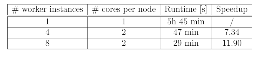
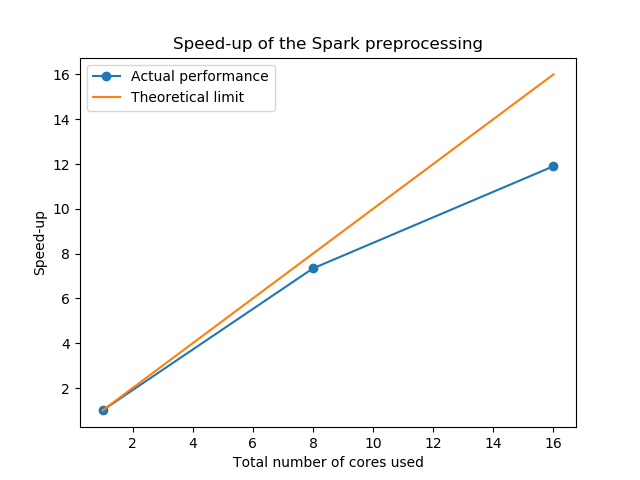
For the cluster, we chose m4.xlarge EC2 instances for both the master node as well as the worker nodes. Each of these have 4 vCPUs, which enables us to parallelize both on the node as on the core level. Different experiments have been run, using multiple nodes and cores, in order to evaluate the achieved speed-up. The following table summarizes the results:
Clearly, the Spark implementation of the patent preprocessing performs well. For an increasing total number of cores used in the parallelization, the speed-up increases and gets reasonably close to the maximal theoretical speed-up. Note that the curve will plateau for increasing number of cores, as the additional overhead cost will become relatively larger compared to the computational gain of an additional core. Using 8 worker nodes and 2 cores per node, the algortihm was eventually able to achieve a speed-up of approximately 12, while the theoretical is 16. As such, the runtime has been reduced to a reasonable 29 mins.
Parallel CGS Implementation
We implemented the parallel approach outlined above using a combination of MPI and OpenMP. As explained in the section on the serial implementation, the vanilla CGS algorithm has a time complexity of O(d\*w) because it involves iterating over every document in the corpus and every word in each document. The purpose of using MPI is to parallelize the processing of the documents, while the purpose of using OpenMP is to parallelize the processing of the words. Because each of these tools was used to parallelize a different part of the CGS algorithm, they are orthogonal to one another and we discuss them separately.
MPI
First, each node reads in an equal number of the partitions output by the Spark program. Because there are 32 partitions in total, this means that two nodes would each read in 16 partitions, four nodes would each read in 8 partitions, etc. Next, each node initializes its document-assignment count and its local word-assignment and topic-assignment counts to zero. Next, an outer loop iterates through each document d and an inner loop iterates through each word w that appears at least one time in the given document. In this inner loop, each occurrence of word w is randomly assigned to one of the topics and the counts are updated accordingly. Additionally, each node keeps track of the fact that document d contains the word w. This saves time later on when the nodes process the word tuples, as they can jump immediately to the relevant documents rather than having to check every document to see if the given word appears in it.
After this nested loop is completed, the nodes need to communicate with each other how they assigned each of the words in their respective documents. First, each node needs access to the global topic-assignment count. This is achieved by calling the MPI_Allreduce function with the MPI_SUM operation, which adds up each node's local topic-assignment count and returns a copy of the resulting count to each of the nodes. Secondly, in preparation of the first iteration, each node requires a queue of word tokens. This is accomplished by splitting up the vocabulary size into N equally sized chunks, where N is the number of nodes. For each batch of words, the MPI_reduce function is called with the MPI_SUM operation. This adds up each node's local word-assignment counts for the relevant words and returns the resulting count to the nth node. At this point, the initialization step has been completed and the first iteration is ready to begin. Note each iteration is composed of N batches, where a batch involves processing all the tuples in the queue, such that each node processes every word in the vocabulary once per iteration.
As explained above in the parallel approach section, each node pops a tuple off of its queue, processes the word and then sends an updated tuple to the next node. While this approach could be implemented such that all communication is asynchronous, there are two major drawbacks to this approach. First, sending and receiving each individual tuple would result in a large overhead cost, with communication happening very often. And second, while this approach would initially work, the algorithm would eventually run into issues as the size of the various queues would become increasingly unbalanced to the point where some nodes have very few tuples while others are swamped with many more than they were initially expected to have. Beyond slowing things down, this lack of coordination could eventually lead to a deadlocking situation that prevents the algorithm from running at all.
Fortunately, upon receiving a tuple, the next node would simply push it onto its own queue. This means the node doesn't need immediate access to this tuple. Therefore, a more efficient approach would be for each node to process multiple tuples and then send this batch of tuples to the next node. However, while this approach would undoubtedly reduce the communication overhead, it would still lead to workload imbalance issues and deadlocking. (We know this from experience as we initially tried this approach and encountered a lot of issues stemming from the lack of synchronization among the nodes.)
It turns out that the optimal communication protocol is also the simplest. Rather than sending individual tuples or sets of tuples to the adjacent node during each batch, the best strategy is to only send sets of tuples when the batch is over (at which point they are free to send their entire set of tuples). At this point, the MPI_Sendrecv function is called, which, for each node, sends the queue of updated tuples to the node to the right and receives the next queue of tuples from the node to the left. (The MPI_Sendrecv function is equivalent to an MPI_Isend and an MPI_Irecv followed by an MPI_Wait for the MPI_Isend and a separate MPI_Wait for the MPI_Irecv.)
There are three advantages of this approach. First, it is much simpler than the other approaches as it doesn't require nodes to constantly call the MPI_Iprobe function to first check if the node to the left has sent a message, and, if a message has arrived, receive the tuples and push them to its queue. Second, this approach involves only one communication event per batch and thus minimizes the communication overhead. And finally, because the MPI_Sendrecv function is a blocking operation, each node cannot proceed until it has sent its queue off to the node to the right and received its new queue from the node to the left. This means that MPI_Sendrecv essentially serves the additional role of MPI_Barrier and ensures that all of the nodes are synchronized before starting the next mini-iteration. This, in turn, guarantees that there are no deadlocking conditions.
The last major detail about the MPI implementation for each mini-iteration is that immediately before the call to MPI_Sendrecv, the MPI_Allreduce function is called with the MPI_SUM operation. This adds the net change topic-assignment counts of each node and sends the result back to each of the nodes so they all have an updated view of the global topic-assignment count.
These batches are carried out until a full iteration (i.e. N batches, where N is the number of nodes) has been completed. At this point, the topic coherence needs to be calculated to check if the CGS algorithm has converged. To calculate the topic coherence for a given topic, we need the M most common words for that topic, and the number of documents in which each pair of these words both occur. To calculate the M most common words, each node first calculates the M most common words among the subset of words that the node has possession over. Then these results can be combined with other nodes’ results in a reduce operation, where the output of two lists of words of length M, sorted by the number of assignments, is a sorted list of length M containing the M common words (this is a partial merge in the classic merge sort algorithm). This was implemented in MPI using a custom MPI_Type (which represents that both the count and the word are sent, as well as the number of words M that are sent); a custom MPI_Op implementing the reduction in-place; and a call to MPI_Allreduce so each node knows the M most common words in each topic. Next, to get the number of documents in which a pair of words occurs for all possible pairs, each node calculates this value for the documents that it has access to. Finally, this information is added together and sent to the master node with a call of MPI_Reduce with the MPI_SUM operation, and the master node calculates the topic coherence.
OpenMP
While the MPI implementation is certainly more efficient than the serial implementation, there is still room for improvement. In particular, each node processes only one tuple at a time, while the rest of the tuples sit idly in the queue. This serial component of the algorithm presents a great opportunity for further parallelization.
To exploit this, we use OpenMP to create multiple threads that each process a tuple at the same time. When a thread finishes processing a tuple, it simply pushes it to the second queue and pops the next tuple off of the primary queue. In Cython, this is achieved by calling the prange function, which takes in a range just as in Python, an argument that sets the number of threads, arguments that specify the schedule and chunksize and a nogil flag that needs to be set to True for OpenMP to run. Because the queue is implemented using a Numpy array, the range is simply the length of the array. Meanwhile, the optimal schedule is dynamic with a chunk size of 1, which allows each node to request the next tuple when it has completed processing the one at hand.
As usual, there is one main benefit and drawback of the dynamic scheduling system. The benefit is that once the final tuple is popped from the queue, the longest the node must wait is the time that it takes to process one word. This contrasts with static and guided scheduling, where the node may have to wait a significant amount of time for a subset of the threads to finish processing the tuples assigned to them, while the rest of the threads have finished their assigned tuples. However, the drawback is that the process of assigning each tuple to a thread has an associated overhead; because the number of assignments in dynamic scheduling is equal to the length of the queue (as opposed to, say, static scheduling where the number of assignments is equal to the number of threads, which is significantly lower than the length of the queue), it has the largest overhead cost out of the three scheduling systems. In this case, however, the number of assignments (i.e. on the order of hundreds of thousands or 10^5) is relatively small. This means that the benefit of dynamic scheduling of reduced idle time outweighs the drawback of increased overhead.
Finally, we need to make sure that multiple threads don't access the same memory simultaneously. Because each thread processes a different word, there is no risk of a conflict for the word-assignment counts. However, at any given time, multiple threads may be reassigning words from the same document and are likely reassigning words to and from the same topic. This means that these threads may try to modify the document-assignment count and the topic-assignment count at the same time. To prevent this from happening, we insert a lock using omp_set_lock in two places: before the topic reassignment when the corresponding document-assignment count and topic-assignment count are decremented, and after the topic reassignment when the corresponding document-assignment count and topic-assignment count are incremented.
Infrastructure & Reproducibility
We chose to run the parallel implementation of the CGS algorithm on a cluster of AWS EC2 instances. The cluster was set up using 1 master node and up to 8 worker nodes, all of which are c4.xlarge instances, which have 4 vCPU, 2.9GHz Intel(R) Xeon(R) CPU E5-2666 v3 processors, 25600K L3 cache, and 7.5 GB memory. Each instance is running Ubuntu 18.04 with the following software:
Python 3.6
Cython 0.29.17
gcc/g++ 7.5.0
MPICH 3.3a2
OpenMP 4.5
For MPI, it is crucial for the cluster set-up to allow the different instances to send and receive information between one another. This can be established with an interconnected virtual private network, which can easily be configured on AWS. After launching all the instances, we create a remote secure interconnection by generating SSH keys and making sure that these are listed under the authorized keys of the worker instances and the master node. Lastly, a shared data storage system is established by configuring an NFS-server and mounting one shared directory to all nodes.When the cluster is set-up correctly, the parallel implementation of the CGS can be run. The overall procedure to do so is summarized in the README-file on Github here .
Performance
The CGS algorithm was run on the Google PATENT dataset using a cluster of AWS EC2 c4.xlarge instances, as described above. The code and instructions in a README can be found here . See cgs.pyx for implementation and main.py for usage. Below is a table of the running time; note we chose to use 16 topics and that the experiments run on one MPI node were done in a c4.2xlarge (which was scaled down to have the same 4 vCPU count using 2 cores and 2 threads per core and running the same operating system and software libraries) because of the larger 15 GB memory.
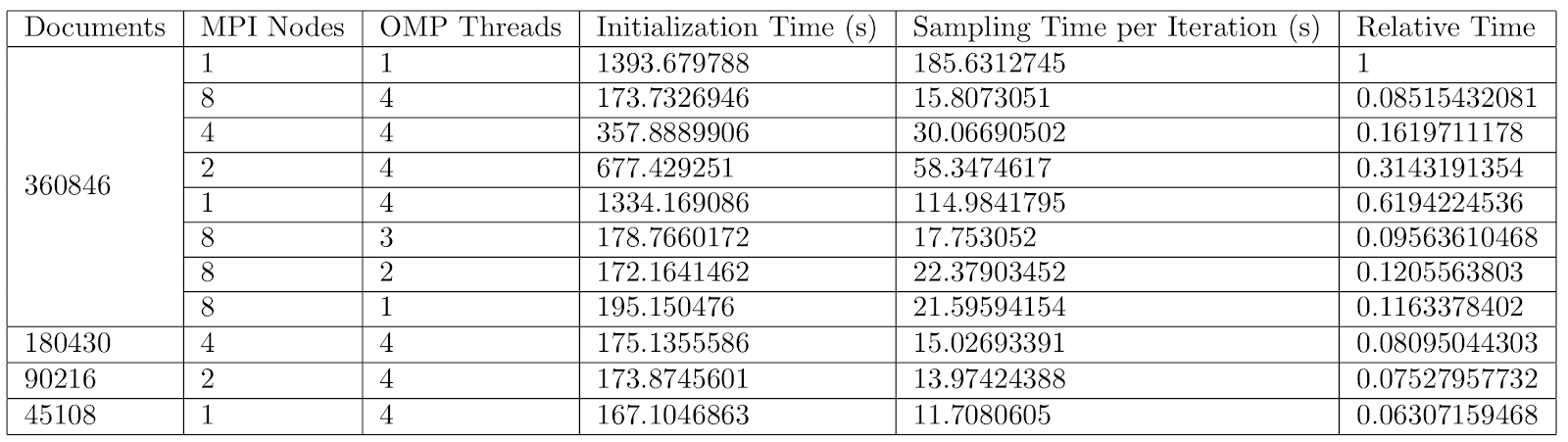
Speedup when using 4 OMP threads, 360,846 documents, and 16 topics.
As shown above, the speedup scales almost linearly with the number of MPI nodes. This makes sense because the ratio of communication to computation is so low. As explained in the implementation section, the only time that the nodes communicate with each other is at the end of each mini-iteration where they exchange tuples and topic-assignment counts; the rest of the time is spent reassigning each of the tuples in the queue. Overall, this means that the speedup increases as the number of documents in the corpus increases, as the communication overhead becomes more and more insignificant relative to the computation as the workload assigned of each node increases.
Speedup when using 8 MPI nodes, 360846 documents, and 16 topics.
The speedup for various number of OMP threads is far from linear and even temporarily decreases when two OMP threads are used. When four threads are used, the speedup only increases to around 1.35. There are several explanations for this lackluster performance. First, it’s possible that the overhead associated with dynamically scheduling the hundreds of thousands of words in each batch is much more significant than we initially thought. However, a higher than expected assignment overhead probably doesn’t account for most of this lack of speedup. A more likely reason for the inefficiency is that, as we explained in the implementation section, we needed to use locks to ensure that only one node has access to the document-specific and topic-specific counts. Because there are so many documents in the corpus, the probability of a collision in the same document is quite small; however, because we chose to only use 16 topics, the probability of a collision in the same topic is much higher and likely occurs many times during each batch. The fact that there are two sets of locks per tuple assignment only compounds this probability of a collision. Therefore, it’s likely that the threads spend a sizable portion of the time waiting to acquire the lock on these assignment counts.
Speedup when using 8 MPI nodes, 360846 documents, and 16 topics.
Scaled speedup has a slope that is significantly less than 1. While communication is relatively infrequent, this can partially be explained by the reduction operations that occur at the end of each iteration, which certainly cannot be completely parallelized.
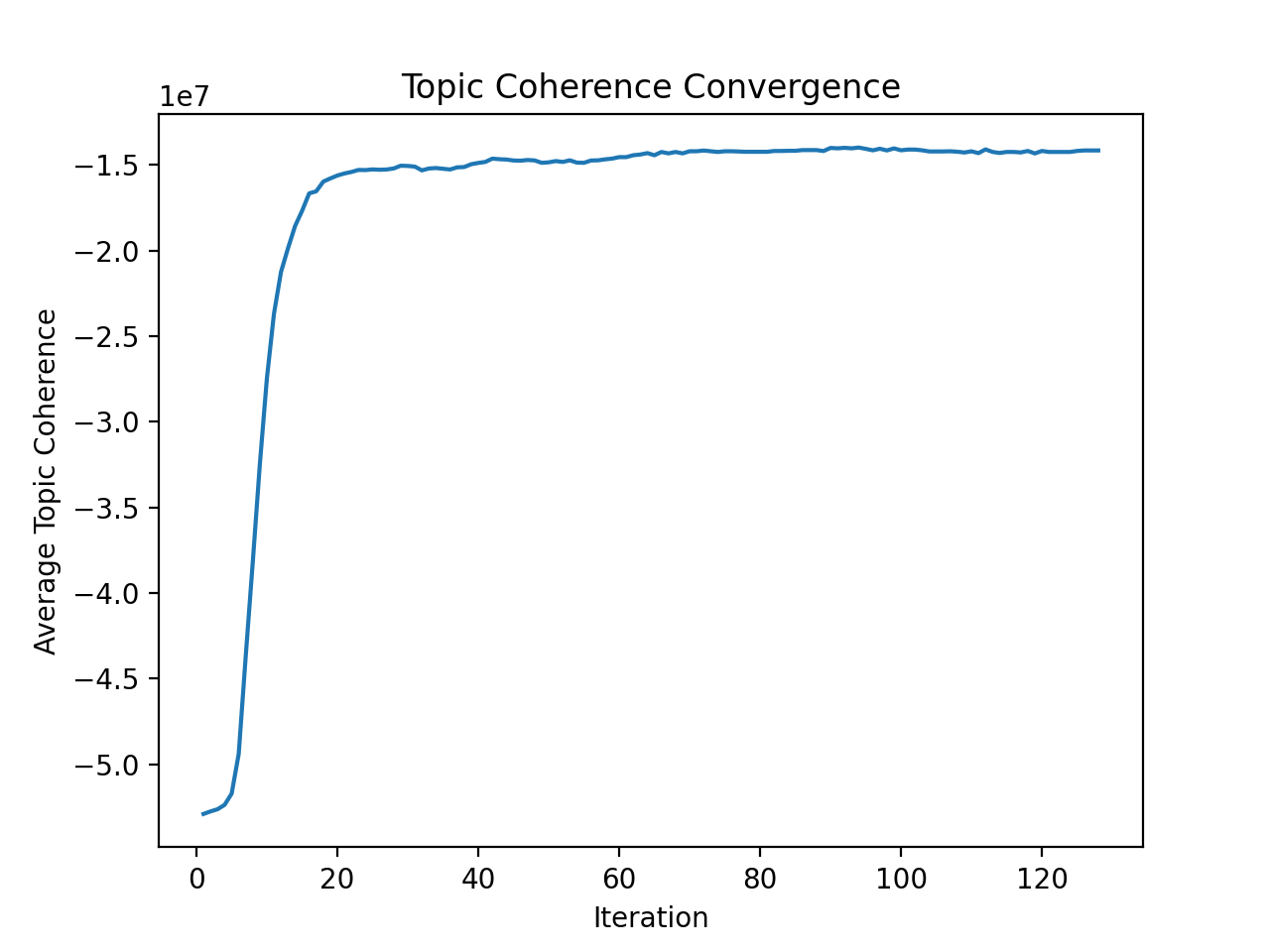
Caption: Average topic coherence on the chosen 360846 document subset of the Google PATENT dataset (run with 8 MPI nodes, 4 OMP threads per node)
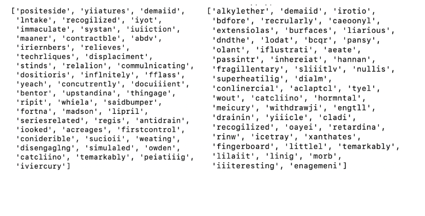
We also evaluated the average topic coherence to ensure that the modified CGS still converges. Note it seems to reach a relatively stable set of assignments in about 50 iterations. However, the actual topic results poorly represent topics as humans would describe them. This is likely due to two reasons: we chose very few topics for the sake of investigating computation time of the algorithm, and the OCR frequently failed, which corrupted the dataset. Below are two examples of the 50 most common words of two topics.
Discussion
Overall, we achieved most of our goals in this project. First, we were able to successfully implement a serial version of CGS. Then, we were able to substantially speed up the preprocessing of the patent documents by using Spark. In terms of the parallelized version of CGS, the MPI implementation performed as well as we could have possibly expected, as it resulted in a nearly linear speedup. The only part that underperformed was our OpenMP implementation, as it didn’t produce much of a speedup over the version that only used MPI. As we’ve explained, this is most likely due to the locks on the document and topic-assignment counts that frequently force the threads to wait for the locks to be freed.
There are several ways that we could address this locking issue. First, we could simply increase the number of topics that we want to infer from the corpus, as this would reduce the probability of two threads trying to modify the counts at the same time. A second, complementary approach would be to avoid locks altogether and instead have each node keep track of its own document and topic-assignment count. After each batch is over, these local net change counts could then be summed together using an OpenMP reduction clause to calculate the overall change in the document and topic-assignment counts. This approach is analogous to the one we used to update the topic-assignment counts among all the nodes after each batch. While this strategy would likely produce a higher speedup as it eliminates any locking issues, the downside is that each thread in a node wouldn’t have access to the precise document and topic-assignment counts. However, the discrepancy between each thread’s local counts and the true global counts should be relatively small, such that the distortion to the categorical distribution is kept to a minimum. Ultimately, testing would need to be done to verify if this is a superior strategy.
One major lesson we learned from this project is to keep the MPI approach as simple as possible and keep the nodes as synchronized as possible. As described in the implementation section, we initially tried to send batches of processed tuples to the next node in the middle of each mini-iteration. After each word was processed by a node, this involved checking if the number of processed tuples exceeded a predefined threshold (we used 25% of the length of the original queue). If this condition was satisfied, these processed tuples were sent to the node to the right as an array. On the flip side, before each word was processed by a node, this involved checking if the node to the left had sent a message. If this condition was met, the message was received and the resulting array was appended to the node's queue. When we tested this complicated implementation, it initially worked fine for the first five or so iterations -- each node was processing its queue at roughly the same pace and all the tuples were transferred successfully between nodes.
However, the algorithm slowly began to break down after this point, as minor discrepancies in the rate at which each node processed its tuples became more and more pronounced. Eventually this created an imbalance where one of the queues contained significantly more tuples than it was supposed to have, and the rest of the nodes had much shorter queues to process. This imbalance and inefficiency grew larger and larger as the rest of the nodes quickly processed their tuples and became idle, while the overwhelmed node had a harder and harder time keeping up. We then tried to prevent this imbalance from taking place by instructing any node whose queue was abnormally long to send the surplus tuples to the node to the right. However, this haphazard solution didn't end up helping. There were also other issues with this implementation that are too subtle to describe but were just as frustrating and difficult to resolve.
Eventually, we realized that there must be a better way to transfer tuples between the nodes. After taking a step back, it didn't take us long to come up with the simple strategy that we ended up using. In retrospect, we realized that MPI programs are supposed to be straightforward to the point where the programmer knows exactly what each node is doing at any given time and there is no complicated control flow logic involving MPI-related tasks. Otherwise, the programmer is likely to experience a cascade of issues that are very difficult to debug and are unpredictable because of the stochastic nature of synchronization problems.
In terms of future work, there are a couple of paths to explore. First, we realize that the code, despite being heavily parallelized already, can still be optimized. For instance, the initialization for the CGS and the computation of the topic coherence still heavily rely on Python. This code could be further optimized by writing it in Cython. Next, the dataset did not seem to be ideal in the end. Although we expected to find a reasonable and relevant topic distribution for the large patent corpus, it appeared that the data had significant flaws. The patents were actually scanned and converted to text using Optical Character Recognition (OCR), which, especially for the older patents, led to meaningless words. As this clearly reduces our ability to intuitively interpret the resulting topics, another dataset might be worth exploring. Lastly, the concept of LDA has recently reached other domains than Natural Language Processing as well. For instance in computer vision, LDA can serve as a natural way for unsupervised image object classification [6]. As these applications can be very computationally expensive as well, it could be worthwhile to expand our parallelization efforts to other domains.
Citations
[1] D. M. Blei, A. Ng, and M. Jordan. “Latent Dirichlet allocation”. Journal of Machine Learning Research, 3:993–1022, Jan. 2003.
[2] D. Minmo, H. M. Wallach, E. Talley, M. Leenders, and A. McCallum, “Optimizing Semantic Coherence in Topic Models,” in Proceedings of the Conference on Empirical Methods in Natural Language Processing, 2011
[3] H.-F. Yu, C.-J. Hsieh, H. Yun, S. V. N. Vishwanathan, and I. S. Dhillon, “A Scalable Asynchronous Distributed Algorithm for Topic Modeling,” in Proceedings of the 24th International Conference on World Wide Web - WWW ’15, 2015, doi: 10.1145/2736277.2741682.
[4] D. M. Blei, Latent Dirichlet Allocation in C. [Online]. Available: http://www.cs.columbia.edu/~blei/lda-c/.
[5] C. Ré, and C. Zhang. DeepDive open datasets, 2015. [Online]. Available: http://deepdive.stanford.edu/opendata
[6] X. Wang, and E. Grimson. "Spatial latent dirichlet allocation." Advances in neural information processing systems, 2008.